
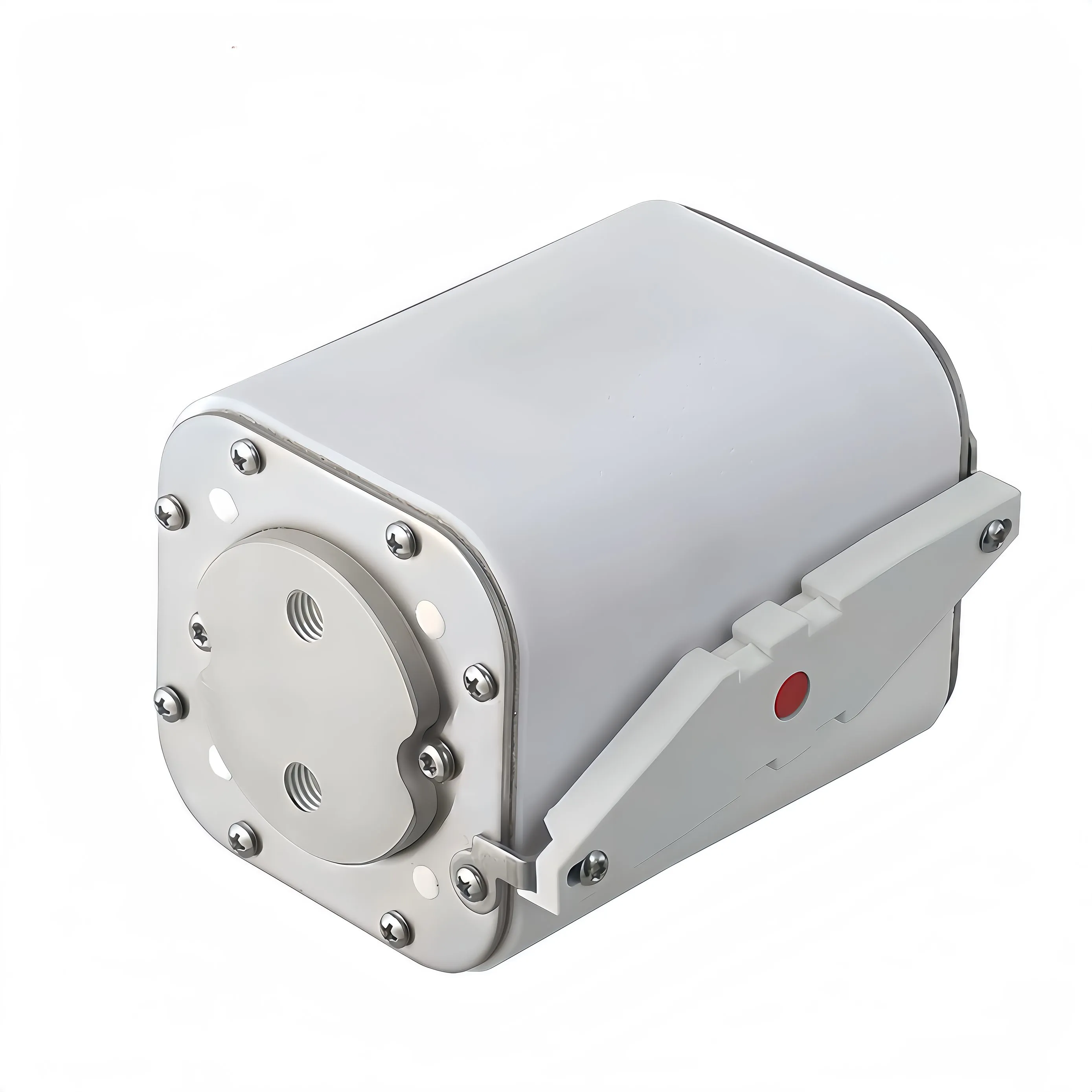
The time-current curve is the most useful sheet of paper in a high speed fuse datasheet, and the one most often skipped. Buyers look at rated current, glance at voltage, and move on. Then a drive trips, a diode fails, and nobody can explain why a device that was supposed to be fast took several milliseconds to clear. The answer was on the curve the whole time. This article is a practical guide to reading that curve properly, including the parts that are easy to misread.
What the Two Axes Really Represent
A time-current curve plots prospective current on the horizontal axis and operating time on the vertical axis. Both axes are logarithmic, which is the first thing to internalise, because a logarithmic plot compresses the region you care about most. The horizontal axis is prospective current — the current that would flow if nothing interrupted it. It is not the current your load draws. A 100 A device protecting a converter that normally draws 60 A is read at the fault current of the system, which might be 20 kA, not at 60 A. The vertical axis is time from fault inception. Depending on which curve you are reading, that time ends either when the element starts to melt or when the current finally reaches zero. Those are different endpoints, and mixing them up is the most common reading error.
Why the Curve Is a Band, Not a Line
Manufacturers draw a band rather than a single line because there is manufacturing tolerance and there is a difference between cold and hot starting conditions. The upper boundary is typically the maximum operating time, and the lower boundary the minimum. When you are checking that a device will protect something, read the upper boundary — the pessimistic case. When you are checking that it will not nuisance-trip on inrush, read the lower boundary — the optimistic case. Using the wrong edge of the band gives you a false sense of margin in one direction or the other. Some datasheets publish separate curves for cold start and for a device already carrying rated current. A warm element melts sooner, so if your equipment cycles continuously, the pre-loaded curve is the honest one to use.
Pre-Arcing Time Versus Total Clearing Time
Two curves usually appear on the same chart, and they are not interchangeable. Pre-arcing, or melting, time runs from fault inception to the point where the element begins to melt. This is the curve you use when comparing against the surge rating of a semiconductor, because the protected device sees rising current throughout this period. Total clearing time adds the arcing period — the time the device spends extinguishing the arc before current reaches zero. This is the curve you use when you are worried about thermal damage to the busbar, the holder, or the enclosure, because energy is still being delivered throughout the arcing period. The gap between the two curves narrows as current rises, because at high prospective current the device operates in a strongly current-limiting mode and both intervals become very short. At low multiples of rated current the gap can be substantial.
Reading the Curve at Your Prospective Current
Here is the procedure, in order:
- Calculate or measure the prospective fault current at the point of installation
- Find that value on the horizontal axis
- Read up to the pre-arcing curve and note the time, using the upper boundary for a protection check
- Multiply out the current squared and the time to get the energy, or read the published I2t curve if one is provided
- Compare that energy with the withstand of the device being protected
- Repeat using the total clearing curve if you are also checking thermal burden on downstream hardware
If your prospective current falls at the far left of the chart, be careful. In the region just above rated current, operating times run to seconds or minutes and depend strongly on cooling conditions, mounting, and the starting temperature of the element.
The Let-Through Charts That Come With It
A time-current curve tells you when the device operates. It does not tell you what the downstream circuit experienced. For that you need two companion charts. The cut-off current chart plots peak let-through current against prospective current. Read it at your fault level and you get the actual peak current your semiconductors and busbars will see — often far below the prospective value, because a fast device begins limiting before the fault current reaches its theoretical maximum. The let-through I2t chart does the same for energy. This is the number you compare against the surge rating of the protected semiconductor. Reading all three charts together is what turns a datasheet into an engineering decision. Reading only the time-current curve leaves out the two quantities that determine whether the silicon survives.
A Worked Example
Suppose a DC link has a prospective fault current of 12 kA and you are protecting a rectifier whose surge withstand is published as an I2t figure. Look up 12 kA on the horizontal axis of the time-current curve. Read the pre-arcing time at the upper boundary — say 0.8 ms. Now look at the let-through I2t chart at the same 12 kA and read the published value directly rather than calculating it, because the current is not constant during the interval. Compare that value with the rectifier's withstand. If the fuse figure is lower with margin, the coordination works. If not, you need a faster or smaller device, or a different class. Repeat the exercise at the lowest fault current your system can produce, not just the maximum. Devices that clear beautifully at 12 kA can be slow and destructive at 800 A, and a bolted fault is not the only fault that happens.
Mistakes We See When Curves Are Read in a Hurry
Reading the axes linearly when they are logarithmic is the classic one, and it makes fast devices look impossibly fast. The second is checking only the maximum fault case. The third is comparing an AC-derived curve against a DC application, where there is no zero crossing to assist interruption. The fourth is forgetting that the curve is valid at a stated ambient temperature; a hot cabinet shifts behaviour.
Summary
The time-current curve answers the question of when. The cut-off and let-through charts answer the question of how much. Read the pre-arcing curve against the semiconductor withstand and the total clearing curve against the thermal burden on the hardware, use the pessimistic edge of the band for protection checks, and always work from the actual prospective current rather than the load current.
About Our High Speed Protection Range
GFEFUSE is the brand of Dongguan Gongfu Electronics Co., Ltd., an electronic protection device manufacturer founded in Dongguan, Guangdong in 2013. We run five advanced production lines with a thirteen-person R&D team, and our products are exported to customers overseas. Our square high speed fuse series covers fast DC protection for drives, converters, and power electronics, with published time-current and let-through data to support coordination studies. For semiconductor protection within the same cabinet we also supply a dedicated North American semiconductor fuse range, and our high voltage fuse portfolio extends protection to the rest of the DC distribution chain. Applications that combine traction and fast DC protection often reference our EV fuse range as well. Products carry UL, cULus, TUV, CE, and CQC certification and comply with RoHS and REACH directives, serving consumer electronics, automotive electronics, power equipment, communication systems, and new energy.
Conclusion
A high speed fuse earns its name in the first few hundred microseconds of a fault, and the datasheet curve is where that behaviour is documented. Once you know which edge of the band to read, which endpoint the curve describes, and which companion chart answers the energy question, the selection stops being guesswork and becomes something you can defend in a design review.
Send us your system voltage, prospective fault current, and the I2t withstand of the device you are protecting. We will read the curves with you and recommend a rating and class.
Frequently Asked Questions
Quick answers on reading the curves that come with a high speed fuse datasheet.
How do you read a high speed fuse time-current curve?
Find your prospective fault current on the horizontal axis, read up to the pre-arcing curve for protection checks, and use the upper boundary of the band for the pessimistic case. Then use the cut-off and let-through I2t charts to see what the downstream circuit actually experiences.
What is the difference between pre-arcing and total clearing time?
Pre-arcing time ends when the element begins to melt, and it is compared with the surge rating of the protected semiconductor. Total clearing time adds the arcing period, and it is used when checking thermal stress on busbars, holders, and enclosures.
Why is the curve drawn as a band?
Because of manufacturing tolerance and the difference between a cold start and a device already carrying current. Use the upper boundary when checking that protection will operate, and the lower boundary when checking that it will not nuisance-trip.
Can I use an AC time-current curve for a DC application?
Not without confirmation. DC has no zero crossing, so arc extinction is harder and behaviour differs. Use data published for your actual voltage type and confirm the time constant of your fault loop against the test conditions.
What is cut-off current on a high speed fuse chart?
It is the peak current the circuit actually sees during interruption, plotted against prospective current. A fast current-limiting device begins limiting before the fault reaches its theoretical peak, so the cut-off value is often far below the prospective value.